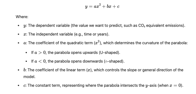
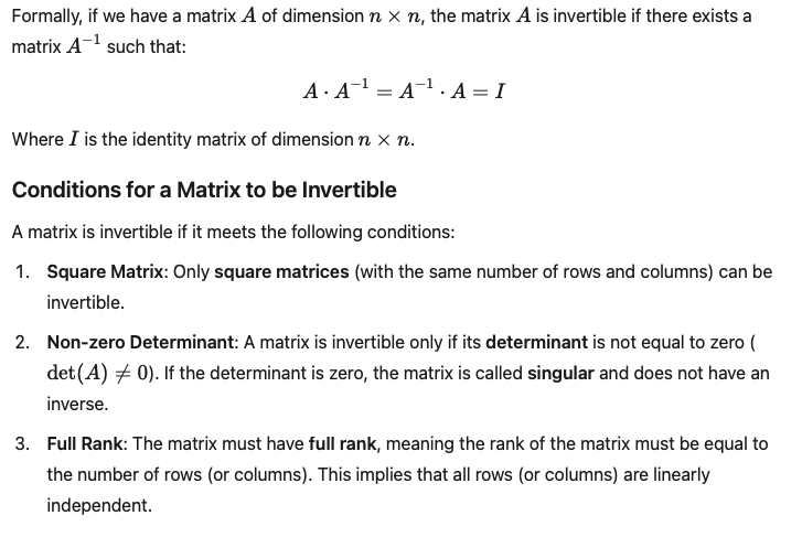
MATHEMATICAL METHOD TO CALCULATE A QUADRATIC REGRESSION TO DETERMINE THE TREND OF CO₂E EMISSIONS IN CATALONIA.
Introduction.
To calculate the evolution of emissions beyond 2023, as explained in the post “Energy Transition in Catalonia: A Look at the CO₂e Emissions History Over the Last 34 Years” it has been deemed appropriate to use the method of quadratic regression to analyze greenhouse gas emissions trends by modeling them in three different periods (1990-2023, 2014-2023, and 2019-2023) for which real total emissions data are available. These data come from greenhouse gas emissions measurements reported by EDGAR (Emissions Database for Global Atmospheric Research), which can be accessed at the following link:
https://edgar.jrc.ec.europa.eu/dataset_ghg2024_nuts2
Specific data for this region were selected from the EDGAR database to analyze emissions in Catalonia. This database includes emissions of various greenhouse gases: CO₂ (carbon dioxide) from fossil sources, CH₄ (methane), N₂O (nitrous oxide), and F-gases (fluorinated gases). By summing the annual emissions of each gas and expressing them in terms of total equivalent CO₂ emissions (in kilotons), the total greenhouse gases generated annually in Catalonia between 1990 and 2023 are obtained. It is worth noting that this annual total lacks a small additional quantity corresponding to the annual secondary emissions of a series of greenhouse gases not recorded by EDGAR. The EDGAR (Emissions Database for Global Atmospheric Research) database focuses on the major greenhouse gases regulated by the Kyoto Protocol, but does not comprehensively cover all possible greenhouse gases.
Thus, using the annual data on CO₂e emissions, Graph 1 is generated. In this graph, one can see how these emissions have evolved from 1990-2023. This graph served as the starting point for analyzing the future emissions trends in Catalonia from 2024 onwards.

An essential aspect of data processing mentioned in the article is that to conduct a thorough analysis, it is necessary to eliminate the data for 2020, as that year, marked by the COVID-19 pandemic, shows an abnormal drop in emissions. Including this value could generate a significant bias in the calculations and affect the results of the future emissions trend.
As can be seen in Graph 1, the data show a non-linear trend in CO₂e emissions over the last 34 years. In this context, as mentioned earlier, to estimate emissions in the coming years, given the characteristics of this small study, performing a quadratic regression using the annual CO₂e emissions data is an appropriate option to model the system and estimate the evolution of emissions in the coming years.
Method for Calculating a Quadratic Regression.
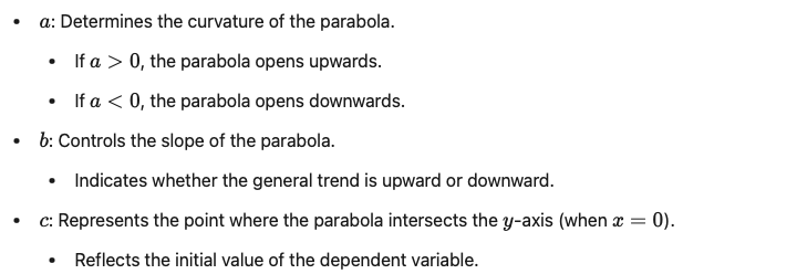
Quadratic regression is a widely used statistical method for its simplicity in finding a relationship between two variables: an independent variable X (in this case, years) and a dependent variable Y (CO₂e emissions). This method is very useful for predicting behaviors, especially when this relationship is not linear but follows a curved shape. It is a simple but powerful statistical tool for analyzing data with non-linear trends. It is especially useful when capturing complex patterns and better understanding trends without delving into more complex multivariable models.
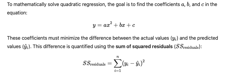
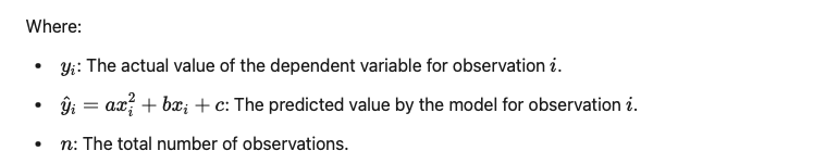
The goal of performing a quadratic regression using the available data is to fit these data to a function in the form of a parabola that best fits the data and minimizes the error between the actual values and the predicted values by the model. This is achieved through the least squares method, which calculates the coefficients (a, b, and c) of the quadratic regression equation, ensuring the total difference between the actual data values and the predicted values (error) is minimized.
The following equation represents the parabolic equation of a quadratic regression:
Objective of the Quadratic Regression Method
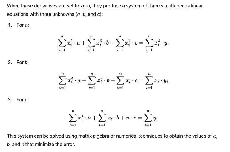
Step 1: Procedure for Calculating the Quadratic Regression
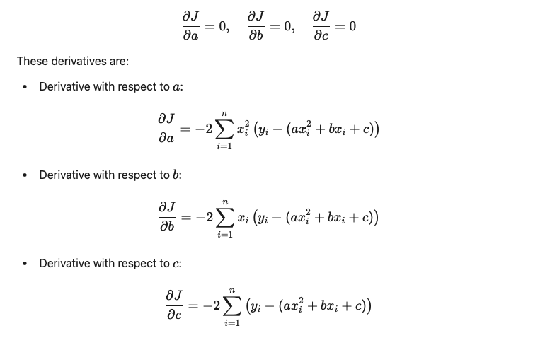
The method used to fit the model is the least squares method, which involves finding the coefficients a, b, and c of the parabolic equation that minimizes the sum of the squares of the residuals. This means the model should aim to make the overall error as small as possible.
The first step is to define what is called the cost function, which is the sum of the squares of the residuals of all the data in the model, that is:

This function J(a, b, c) aims to calculate how well the model fits the real data. In other words, it seeks the values of coefficients a, b, and c that make the cost function J(a, b, c) minimal and best define the quadratic curve that most closely matches the actual data. To achieve this, it is necessary to derive the cost function for each of the coefficients of the parabolic equation and set these derivatives equal to zero. This generates a system of equations that can be solved as follows:
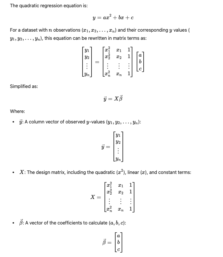
Based on the quadratic regression equation:
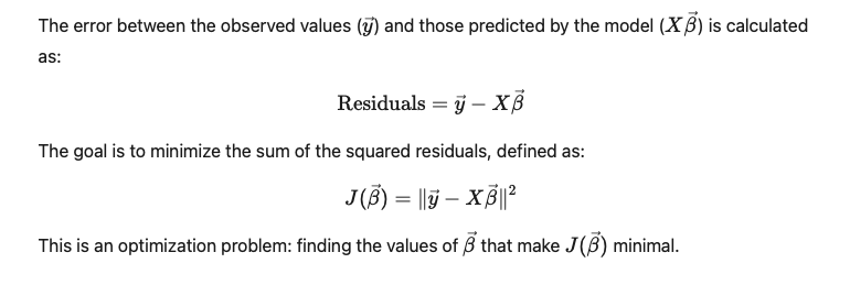
Once the matrix system is established, the next step is to determine, using matrix calculations, the optimal values of the coefficients a, b, and c that minimize the error between the observed values and those predicted by the model.
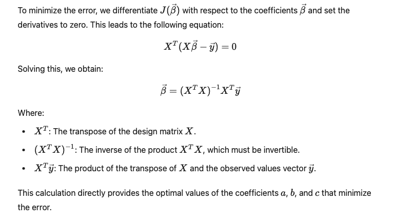
Once it has been determined that the matrix (XTX)-1 is invertible1, and this system is subsequently solved using matrix calculations, the optimal values for the coefficients a, b, and c that minimize the error are directly obtained, as explained earlier:
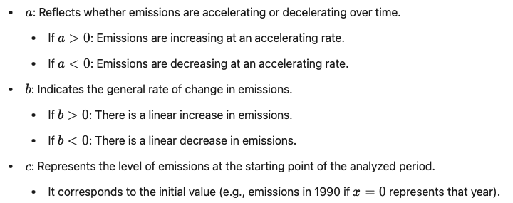
For practical purposes, in our case, for analyzing CO₂e emissions over time, this means:
Step 2: Procedure for Validating the Results Obtained to Ensure That the Models Fit the Actual Data Adequately.
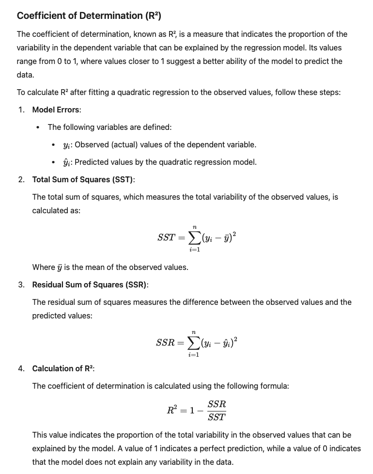
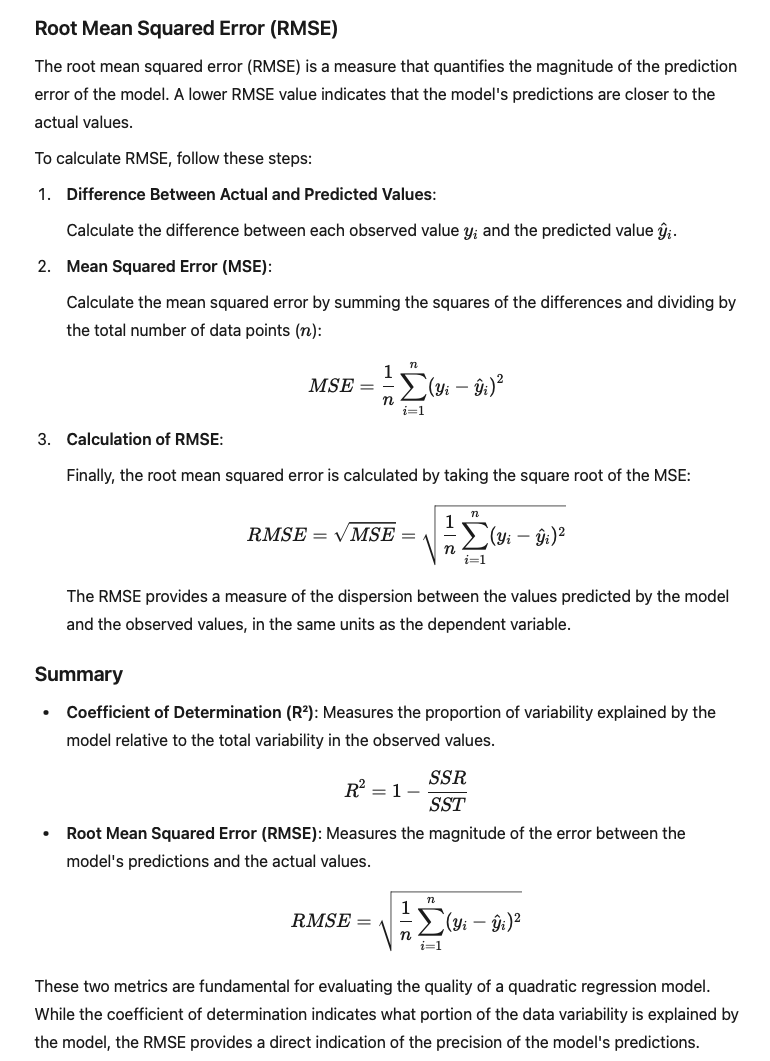
Once the quadratic regression models are calculated, it is essential to validate the results to ensure they adequately fit the actual data. This validation is key to determining with a certain degree of confidence whether the models are appropriate and can be used for reliable predictions. To this end, two methods are used: the coefficient of determination (R²) and the root mean squared error (RMSE).
R² and RMSE are widely used statistical methods to evaluate a mathematical model’s quality. R² (coefficient of determination) indicates what portion of the variability of the actual data is explained by the model. A value close to 1 means the model describes the data well, while a value close to 0 indicates little relation between the model and the actual data. On the other hand, RMSE (Root Mean Squared Error) measures, on average, the model’s prediction error. Expressed in the same units as the data, RMSE shows how far the model’s predictions deviate from the actual values.
In other words, R² helps us understand “how well the model explains the real data,” while RMSE indicates “how accurate the predictions are.” To ensure that the models fit reality and can reliably predict CO₂e emissions trends in the coming years, achieving a high R² and a low RMSE is necessary.
To calculate these two parameters, the following procedure must be followed:
- An invertible matrix means that there is another matrix, called the inverse matrix, which, when multiplied by the original matrix, results in the identity matrix. This property is fundamental in linear algebra and has significant implications in solving systems of linear equations, among other applications.
↩︎